How Do You Know if a Distribution Is Bimodal

Probability distribution whose density has two or more distinct local maxima

"Bimodal" redirects here. For the musical concept, come across Bimodality.

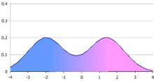
Effigy 1. A simple bimodal distribution, in this example a mixture of ii normal distributions with the same variance but different means. The effigy shows the probability density function (p.d.f.), which is an every bit-weighted boilerplate of the bell-shaped p.d.f.s of the two normal distributions. If the weights were not equal, the resulting distribution could still be bimodal but with peaks of unlike heights.

Figure 2. A bimodal distribution.

Effigy three. A bivariate, multimodal distribution

In statistics, a bimodal distribution is a probability distribution with ii different modes, which may also exist referred to as a bimodal distribution. These appear as distinct peaks (local maxima) in the probability density part, as shown in Figures 1 and two. Categorical, continuous, and discrete data tin all form bimodal distributions^{[ citation needed ]}.

More generally, a multimodal distribution is a probability distribution with two or more modes, as illustrated in Effigy 3.

Terminology [edit]

When the two modes are unequal the larger manner is known as the major mode and the other every bit the minor style. The to the lowest degree frequent value betwixt the modes is known as the antimode. The difference between the major and minor modes is known equally the amplitude. In time series the major mode is called the acrophase and the antimode the batiphase.^{[ citation needed ]}

Galtung's classification [edit]

Galtung introduced a classification system (AJUS) for distributions:^[1]

• A: unimodal distribution – superlative in the middle
• J: unimodal – peak at either end
• U: bimodal – peaks at both ends
• S: bimodal or multimodal – multiple peaks

This classification has since been modified slightly:

• J: (modified) – summit on right
• 50: unimodal – acme on left
• F: no peak (apartment)

Under this classification bimodal distributions are classified as type S or U.

Examples [edit]

Bimodal distributions occur both in mathematics and in the natural sciences.

Probability distributions [edit]

Important bimodal distributions include the arcsine distribution and the beta distribution. Others include the U-quadratic distribution.

The ratio of two normal distributions is also bimodally distributed. Let

${\displaystyle R={\frac {a+x}{b+y}}}$

where a and b are constant and x and y are distributed as normal variables with a hateful of 0 and a standard deviation of 1. R has a known density that can be expressed equally a confluent hypergeometric office.^[2]

The distribution of the reciprocal of a t distributed random variable is bimodal when the degrees of freedom are more than i. Similarly the reciprocal of a normally distributed variable is also bimodally distributed.

A t statistic generated from data set drawn from a Cauchy distribution is bimodal.^[3]

Occurrences in nature [edit]

Examples of variables with bimodal distributions include the fourth dimension between eruptions of certain geysers, the color of galaxies, the size of worker weaver ants, the age of incidence of Hodgkin's lymphoma, the speed of inactivation of the drug isoniazid in Usa adults, the absolute magnitude of novae, and the circadian activity patterns of those crepuscular animals that are agile both in morning and evening twilight. In fishery scientific discipline multimodal length distributions reflect the dissimilar year classes and can thus be used for age distribution- and growth estimates of the fish population.^[4] Sediments are normally distributed in a bimodal fashion. When sampling mining galleries crossing either the host stone and the mineralized veins, the distribution of geochemical variables would be bimodal. Bimodal distributions are as well seen in traffic analysis, where traffic peaks in during the AM rush 60 minutes then once again in the PM blitz hour. This phenomenon is as well seen in daily water distribution, as water need, in the form of showers, cooking, and toilet use, generally peak in the morning time and evening periods.

Econometrics [edit]

In econometric models, the parameters may be bimodally distributed.^[five]

Origins [edit]

Mathematical [edit]

A bimodal distribution well-nigh commonly arises equally a mixture of ii different unimodal distributions (i.e. distributions having just one mode). In other words, the bimodally distributed random variable Ten is divers as ${\displaystyle Y}$ with probability ${\displaystyle \alpha }$ or ${\displaystyle Z}$ with probability ${\displaystyle (ane-\alpha ),}$ where Y and Z are unimodal random variables and ${\displaystyle 0<\alpha <i}$ is a mixture coefficient.

Mixtures with two distinct components need not be bimodal and 2 component mixtures of unimodal component densities can accept more than two modes. In that location is no immediate connection between the number of components in a mixture and the number of modes of the resulting density.

Particular distributions [edit]

Bimodal distributions, despite their frequent occurrence in information sets, accept only rarely been studied^{[ citation needed ]}. This may be because of the difficulties in estimating their parameters either with frequentist or Bayesian methods. Amongst those that have been studied are

• Bimodal exponential distribution.^[6]
• Alpha-skew-normal distribution.^[7]
• Bimodal skew-symmetric normal distribution.^[viii]
• A mixture of Conway-Maxwell-Poisson distributions has been fitted to bimodal count data.^[nine]

Bimodality too naturally arises in the cusp catastrophe distribution.

Biology [edit]

In biological science five factors are known to contribute to bimodal distributions of population sizes^{[ commendation needed ]}:

• the initial distribution of individual sizes
• the distribution of growth rates among the individuals
• the size and fourth dimension dependence of the growth rate of each individual
• mortality rates that may affect each size class differently
• the DNA methylation in human and mouse genome.

The bimodal distribution of sizes of weaver ant workers arises due to beingness of two distinct classes of workers, namely major workers and small workers.^[10]

The distribution of fitness effects of mutations for both whole genomes^{[11] [12]} and individual genes^[13] is also ofttimes constitute to exist bimodal with nigh mutations being either neutral or lethal with relatively few having intermediate effect.

General properties [edit]

A mixture of 2 unimodal distributions with differing means is not necessarily bimodal. The combined distribution of heights of men and women is sometimes used as an example of a bimodal distribution, but in fact the deviation in mean heights of men and women is as well pocket-sized relative to their standard deviations to produce bimodality.^[14]

Bimodal distributions have the peculiar property that – dissimilar the unimodal distributions – the hateful may be a more robust sample estimator than the median.^[15] This is clearly the instance when the distribution is U shaped like the arcsine distribution. It may not be truthful when the distribution has one or more than long tails.

Moments of mixtures [edit]

Allow

${\displaystyle f(x)=pg_{1}(ten)+(1-p)g_{2}(x)\,}$

where g _i is a probability distribution and p is the mixing parameter.

The moments of f(10) are^[16]

${\displaystyle \mu =p\mu _{1}+(i-p)\mu _{2}}$

${\displaystyle \nu _{two}=p[\sigma _{1}^{2}+\delta _{ane}^{2}]+(1-p)[\sigma _{2}^{2}+\delta _{2}^{2}]}$

${\displaystyle \nu _{3}=p[S_{1}\sigma _{1}^{3}+three\delta _{1}\sigma _{1}^{two}+\delta _{ane}^{3}]+(ane-p)[S_{2}\sigma _{2}^{three}+three\delta _{two}\sigma _{2}^{2}+\delta _{two}^{3}]}$

${\displaystyle \nu _{iv}=p[K_{one}\sigma _{1}^{4}+4S_{i}\delta _{one}\sigma _{i}^{3}+6\delta _{1}^{2}\sigma _{1}^{2}+\delta _{1}^{four}]+(1-p)[K_{ii}\sigma _{2}^{4}+4S_{2}\delta _{2}\sigma _{two}^{3}+vi\delta _{ii}^{ii}\sigma _{2}^{two}+\delta _{2}^{4}]}$

where

${\displaystyle \mu =\int xf(x)\,dx}$

${\displaystyle \delta _{i}=\mu _{i}-\mu }$

${\displaystyle \nu _{r}=\int (x-\mu )^{r}f(x)\,dx}$

and S _i and K _i are the skewness and kurtosis of the i ^th distribution.

Mixture of ii normal distributions [edit]

It is not uncommon to encounter situations where an investigator believes that the information comes from a mixture of ii normal distributions. Because of this, this mixture has been studied in some detail.^[17]

A mixture of two normal distributions has five parameters to guess: the 2 means, the two variances and the mixing parameter. A mixture of two normal distributions with equal standard deviations is bimodal simply if their means differ by at least twice the common standard deviation.^[14] Estimates of the parameters is simplified if the variances tin be causeless to be equal (the homoscedastic case).

If the means of the 2 normal distributions are equal, then the combined distribution is unimodal. Conditions for unimodality of the combined distribution were derived past Eisenberger.^[eighteen] Necessary and sufficient atmospheric condition for a mixture of normal distributions to be bimodal have been identified by Ray and Lindsay.^[nineteen]

A mixture of two approximately equal mass normal distributions has a negative kurtosis since the 2 modes on either side of the centre of mass effectively reduces the tails of the distribution.

A mixture of two normal distributions with highly unequal mass has a positive kurtosis since the smaller distribution lengthens the tail of the more dominant normal distribution.

Mixtures of other distributions require additional parameters to be estimated.

Tests for unimodality [edit]

• The mixture is unimodal if and only if^[20]

${\displaystyle d\leq 1}$

or

${\displaystyle \left\vert \log(1-p)-\log(p)\right\vert \geq 2\log(d-{\sqrt {d^{2}-ane}})+2d{\sqrt {d^{2}-1}},}$

where p is the mixing parameter and

${\displaystyle d={\frac {\left\vert \mu _{1}-\mu _{two}\right\vert }{ii{\sqrt {\sigma _{one}\sigma _{two}}}}},}$

and where μ ₁ and μ ₂ are the means of the two normal distributions and σ ₁ and σ ₂ are their standard deviations.

• The following test for the instance p = 1/two was described past Schilling et al.^[14] Let

${\displaystyle r={\frac {\sigma _{1}^{2}}{\sigma _{ii}^{2}}}.}$

The separation factor (S) is

${\displaystyle S={\frac {\sqrt {-2+3r+3r^{two}-2r^{3}+2(ane-r+r^{2})^{1.5}}}{{\sqrt {r}}(1+{\sqrt {r}})}}.}$

If the variances are equal and so S = 1. The mixture density is unimodal if and merely if

${\displaystyle |\mu _{1}-\mu _{ii}|<Southward|\sigma _{1}+\sigma _{ii}|.}$

• A sufficient condition for unimodality is^[21]

${\displaystyle |\mu _{1}-\mu _{2}|\leq 2\min(\sigma _{1},\sigma _{2}).}$

• If the two normal distributions have equal standard deviations ${\displaystyle \sigma ,}$ a sufficient condition for unimodality is^[21]

${\displaystyle |\mu _{1}-\mu _{2}|\leq 2\sigma {\sqrt {i+{\frac {|\log p-\ln(i-p)|}{2}}}}.}$

Summary statistics [edit]

Bimodal distributions are a usually used example of how summary statistics such as the hateful, median, and standard departure can be deceptive when used on an arbitrary distribution. For instance, in the distribution in Figure 1, the mean and median would exist about nada, even though zero is non a typical value. The standard divergence is as well larger than deviation of each normal distribution.

Although several have been suggested, in that location is no presently generally agreed summary statistic (or gear up of statistics) to quantify the parameters of a general bimodal distribution. For a mixture of 2 normal distributions the ways and standard deviations along with the mixing parameter (the weight for the combination) are usually used – a total of v parameters.

Ashman's D [edit]

A statistic that may be useful is Ashman'due south D:^[22]

${\displaystyle D=(2^{\frac {one}{2}}){\frac {\left|\mu _{1}-\mu _{2}\right|}{\sqrt {(\sigma _{ane}^{2}+\sigma _{2}^{2})}}}}$

where μ ₁, μ _two are the ways and σ _i σ ₂ are the standard deviations.

For a mixture of 2 normal distributions D > 2 is required for a clean separation of the distributions.

van der Eijk's A [edit]

This mensurate is a weighted average of the caste of agreement the frequency distribution.^[23] A ranges from -1 (perfect bimodality) to +one (perfect unimodality). Information technology is defined as

${\displaystyle A=U(1-{\frac {S-one}{K-i}})}$

where U is the unimodality of the distribution, South the number of categories that have nonzero frequencies and K the total number of categories.

The value of U is 1 if the distribution has any of the three post-obit characteristics:

• all responses are in a single category
• the responses are evenly distributed amongst all the categories
• the responses are evenly distributed amidst two or more contiguous categories, with the other categories with nothing responses

With distributions other than these the information must be divided into 'layers'. Within a layer the responses are either equal or zero. The categories do not have to be face-to-face. A value for A for each layer (A _i) is calculated and a weighted average for the distribution is determined. The weights (w _i) for each layer are the number of responses in that layer. In symbols

${\displaystyle A_{overall}=\sum w_{i}A_{i}}$

A compatible distribution has A = 0: when all the responses autumn into ane category A = +1.

One theoretical problem with this alphabetize is that information technology assumes that the intervals are equally spaced. This may limit its applicability.

Bimodal separation [edit]

This index assumes that the distribution is a mixture of 2 normal distributions with means (μ _ane and μ _ii) and standard deviations (σ ₁ and σ _ii):^[24]

${\displaystyle S={\frac {\mu _{i}-\mu _{two}}{2(\sigma _{1}+\sigma _{2})}}}$

Bimodality coefficient [edit]

Sarle's bimodality coefficient b is^[25]

${\displaystyle \beta ={\frac {\gamma ^{two}+1}{\kappa }}}$

where γ is the skewness and κ is the kurtosis. The kurtosis is here defined to be the standardised fourth moment around the mean. The value of b lies between 0 and ane.^[26] The logic behind this coefficient is that a bimodal distribution with light tails will have very depression kurtosis, an asymmetric character, or both – all of which increase this coefficient.

The formula for a finite sample is^[27]

${\displaystyle b={\frac {g^{2}+i}{thou+{\frac {3(n-1)^{ii}}{(n-two)(n-iii)}}}}}$

where n is the number of items in the sample, g is the sample skewness and k is the sample backlog kurtosis.

The value of b for the uniform distribution is 5/nine. This is also its value for the exponential distribution. Values greater than 5/9 may indicate a bimodal or multimodal distribution, though corresponding values tin also issue for heavily skewed unimodal distributions.^[28] The maximum value (i.0) is reached but by a Bernoulli distribution with merely 2 distinct values or the sum of ii dissimilar Dirac delta functions (a bi-delta distribution).

The distribution of this statistic is unknown. Information technology is related to a statistic proposed before by Pearson – the difference betwixt the kurtosis and the foursquare of the skewness (vide infra).

Bimodality amplitude [edit]

This is defined equally^[24]

${\displaystyle A_{B}={\frac {A_{ane}-A_{an}}{A_{1}}}}$

where A _one is the amplitude of the smaller tiptop and A _an is the amplitude of the antimode.

A _B is always < 1. Larger values indicate more distinct peaks.

Bimodal ratio [edit]

This is the ratio of the left and correct peaks.^[24] Mathematically

${\displaystyle R={\frac {A_{r}}{A_{50}}}}$

where A ₅₀ and A _r are the amplitudes of the left and correct peaks respectively.

Bimodality parameter [edit]

This parameter (B) is due to Wilcock.^[29]

${\displaystyle B=({\frac {A_{r}}{A_{l}}})^{0.v}\sum P_{i}}$

where A _fifty and A _r are the amplitudes of the left and correct peaks respectively and P _i is the logarithm taken to the base 2 of the proportion of the distribution in the i^th interval. The maximal value of the ΣP is 1 but the value of B may exist greater than this.

To use this alphabetize, the log of the values are taken. The information is then divided into interval of width Φ whose value is log 2. The width of the peaks are taken to be four times ane/4Φ centered on their maximum values.

Bimodality indices [edit]

Wang'south alphabetize

The bimodality index proposed by Wang et al assumes that the distribution is a sum of ii normal distributions with equal variances but differing ways.^[xxx] Information technology is defined as follows:

${\displaystyle \delta ={\frac {|\mu _{1}-\mu _{ii}|}{\sigma }}}$

where μ _one, μ ₂ are the means and σ is the common standard departure.

${\displaystyle BI=\delta {\sqrt {p(i-p)}}}$

where p is the mixing parameter.

Sturrock'southward index

A different bimodality index has been proposed past Sturrock.^[31]

This alphabetize (B) is defined as

${\displaystyle B={\frac {1}{N}}\left[\left(\sum _{1}^{Due north}\cos(2\pi grand\gamma )\right)^{2}+\left(\sum _{one}^{N}\sin(ii\pi yard\gamma )\right)^{2}\right]}$

When m = 2 and γ is uniformly distributed, B is exponentially distributed.^[32]

This statistic is a form of periodogram. It suffers from the usual bug of estimation and spectral leakage common to this form of statistic.

de Michele and Accatino'southward index

Another bimodality index has been proposed by de Michele and Accatino.^[33] Their index (B) is

${\displaystyle B=|\mu -\mu _{Thousand}|}$

where μ is the arithmetic mean of the sample and

${\displaystyle \mu _{One thousand}={\frac {\sum _{i=i}^{50}m_{i}x_{i}}{\sum _{i=i}^{L}m_{i}}}}$

where thou _i is number of data points in the i ^th bin, x _i is the center of the i ^th bin and L is the number of bins.

The authors suggested a cutting off value of 0.i for B to distinguish betwixt a bimodal (B > 0.one)and unimodal (B < 0.1) distribution. No statistical justification was offered for this value.

Sambrook Smith'southward alphabetize

A further index (B) has been proposed by Sambrook Smith et al ^[34]

${\displaystyle B=|\phi _{2}-\phi _{1}|{\frac {p_{2}}{p_{1}}}}$

where p ₁ and p _two are the proportion contained in the primary (that with the greater aamplitude) and secondary (that with the bottom amplitude) mode and φ _one and φ ₂ are the φ-sizes of the main and secondary mode. The φ-size is divers every bit minus i times the log of the information size taken to the base 2. This transformation is commonly used in the study of sediments.

The authors recommended a cut off value of 1.5 with B existence greater than 1.5 for a bimodal distribution and less than one.5 for a unimodal distribution. No statistical justification for this value was given.

Chaudhuri and Agrawal alphabetize

Another bimodality parameter has been proposed by Chaudhuri and Agrawal.^[35] This parameter requires knowledge of the variances of the two subpopulations that make up the bimodal distribution. It is defined every bit

${\displaystyle k={\frac {n_{i}\sigma _{1}^{2}+n_{2}\sigma _{two}^{two}}{m\sigma ^{2}}}}$

where n _i is the number of information points in the i ^thursday subpopulation, σ _i ² is the variance of the i ^th subpopulation, grand is the total size of the sample and σ ² is the sample variance.

Information technology is a weighted average of the variance. The authors suggest that this parameter tin can exist used as the optimisation target to carve up a sample into ii subpopulations. No statistical justification for this suggestion was given.

Statistical tests [edit]

A number of tests are bachelor to determine if a data set is distributed in a bimodal (or multimodal) manner.

Graphical methods [edit]

In the study of sediments, particle size is frequently bimodal. Empirically, it has been establish useful to plot the frequency confronting the log( size ) of the particles.^{[36] [37]} This usually gives a clear separation of the particles into a bimodal distribution. In geological applications the logarithm is normally taken to the base two. The log transformed values are referred to equally phi (Φ) units. This system is known as the Krumbein (or phi) calibration.

An culling method is to plot the log of the particle size against the cumulative frequency. This graph will usually consist two reasonably direct lines with a connecting line respective to the antimode.

Statistics

Approximate values for several statistics tin be derived from the graphic plots.^[36]

${\displaystyle {\mathit {Mean}}={\frac {\phi _{16}+\phi _{fifty}+\phi _{84}}{3}}}$

${\displaystyle {\mathit {StdDev}}={\frac {\phi _{84}-\phi _{16}}{four}}+{\frac {\phi _{95}-\phi _{v}}{6.half dozen}}}$

${\displaystyle {\mathit {Skew}}={\frac {\phi _{84}+\phi _{16}-2\phi _{50}}{ii(\phi _{84}-\phi _{16})}}+{\frac {\phi _{95}+\phi _{5}-2\phi _{50}}{2(\phi _{95}-\phi _{5})}}}$

${\displaystyle {\mathit {Kurt}}={\frac {\phi _{95}-\phi _{five}}{2.44(\phi _{75}-\phi _{25})}}}$

where Mean is the mean, StdDev is the standard deviation, Skew is the skewness, Kurt is the kurtosis and φ _x is the value of the variate φ at the ten ^thursday pct of the distribution.

Unimodal vs. bimodal distribution [edit]

Pearson in 1894 was the first to devise a procedure to test whether a distribution could exist resolved into two normal distributions.^[38] This method required the solution of a 9th gild polynomial. In a subsequent paper Pearson reported that for whatever distribution skewness² + one < kurtosis.^[26] Subsequently Pearson showed that^[39]

${\displaystyle b_{ii}-b_{1}\geq one}$

where b ₂ is the kurtosis and b ₁ is the square of the skewness. Equality holds only for the two point Bernoulli distribution or the sum of two different Dirac delta functions. These are the nigh extreme cases of bimodality possible. The kurtosis in both these cases is 1. Since they are both symmetrical their skewness is 0 and the deviation is 1.

Bakery proposed a transformation to convert a bimodal to a unimodal distribution.^[40]

Several tests of unimodality versus bimodality have been proposed: Haldane suggested one based on second central differences.^[41] Larkin later introduced a exam based on the F test;^[42] Benett created one based on Fisher's G test.^[43] Tokeshi has proposed a fourth examination.^{[44] [45]} A test based on a likelihood ratio has been proposed by Holzmann and Vollmer.^[xx]

A method based on the score and Wald tests has been proposed.^[46] This method tin distinguish between unimodal and bimodal distributions when the underlying distributions are known.

Antimode tests [edit]

Statistical tests for the antimode are known.^[47]

Otsu's method

Otsu'southward method is usually employed in estimator graphics to determine the optimal separation between two distributions.

General tests [edit]

To test if a distribution is other than unimodal, several additional tests take been devised: the bandwidth test,^[48] the dip test,^[49] the excess mass test,^[fifty] the MAP test,^[51] the mode existence examination,^[52] the runt exam,^{[53] [54]} the span test,^[55] and the saddle test.

An implementation of the dip test is available for the R programming linguistic communication.^[56] The p-values for the dip statistic values range between 0 and ane. P-values less than 0.05 indicate pregnant multimodality and p-values greater than 0.05 but less than 0.ten suggest multimodality with marginal significance.^[57]

Silverman's test [edit]

Silverman introduced a bootstrap method for the number of modes.^[48] The examination uses a fixed bandwidth which reduces the ability of the exam and its interpretability. Under smoothed densities may have an excessive number of modes whose count during bootstrapping is unstable.

Bajgier-Aggarwal test [edit]

Bajgier and Aggarwal accept proposed a exam based on the kurtosis of the distribution.^[58]

Special cases [edit]

Additional tests are available for a number of special cases:

Mixture of two normal distributions

A study of a mixture density of two normal distributions data found that separation into the two normal distributions was difficult unless the ways were separated by 4–half-dozen standard deviations.^[59]

In astronomy the Kernel Mean Matching algorithm is used to determine if a data set belongs to a single normal distribution or to a mixture of two normal distributions.

Beta-normal distribution

This distribution is bimodal for certain values of is parameters. A exam for these values has been described.^[sixty]

Parameter interpretation and fitting curves [edit]

Assuming that the distribution is known to be bimodal or has been shown to be bimodal by one or more of the tests above, it is oft desirable to fit a bend to the data. This may be hard.

Bayesian methods may be useful in difficult cases.

Software [edit]

Two normal distributions

A packet for R is available for testing for bimodality.^[61] This package assumes that the data are distributed every bit a sum of two normal distributions. If this assumption is not correct the results may not be reliable. It also includes functions for fitting a sum of two normal distributions to the information.

Assuming that the distribution is a mixture of two normal distributions then the expectation-maximization algorithm may be used to make up one's mind the parameters. Several programmes are bachelor for this including Cluster,^[62] and the R package nor1mix.^[63]

Other distributions

The mixtools package available for R tin can test for and estimate the parameters of a number of different distributions.^[64] A parcel for a mixture of two right-tailed gamma distributions is bachelor.^[65]

Several other packages for R are bachelor to fit mixture models; these include flexmix,^[66] mcclust,^[67] agrmt,^[68] and mixdist.^[69]

The statistical programming language SAS can also fit a variety of mixed distributions with the PROC FREQ process.

Run into too [edit]

• Overdispersion

References [edit]

1. ^ Galtung, J. (1969). Theory and methods of social research. Oslo: Universitetsforlaget. ISBN0-04-300017-7.
2. ^ Fieller East (1932). "The distribution of the alphabetize in a normal bivariate population". Biometrika. 24 (3–iv): 428–440. doi:10.1093/biomet/24.iii-4.428.
3. ^ Fiorio, CV; HajivassILiou, VA; Phillips, PCB (2010). "Bimodal t-ratios: the touch on of thick tails on inference". The Econometrics Journal. 13 (2): 271–289. doi:10.1111/j.1368-423X.2010.00315.ten. S2CID 363740.
4. ^ Introduction to tropical fish stock assessment
5. ^ Phillips, P. C. B. (2006). "A remark on bimodality and weak instrumentation in structural equation interpretation" (PDF). Econometric Theory. 22 (5): 947–960. doi:10.1017/S0266466606060439. S2CID 16775883.
6. ^ Hassan, MY; Hijazi, RH (2010). "A bimodal exponential power distribution". Pakistan Journal of Statistics. 26 (2): 379–396.
7. ^ Elal-Olivero, D (2010). "Alpha-skew-normal distribution". Proyecciones Journal of Mathematics. 29 (3): 224–240. doi:10.4067/s0716-09172010000300006.
8. ^ Hassan, Thousand. Y.; El-Bassiouni, One thousand. Y. (2016). "Bimodal skew-symmetric normal distribution". Communications in Statistics - Theory and Methods. 45 (v): 1527–1541. doi:10.1080/03610926.2014.882950. S2CID 124087015.
9. ^ Bosea, S.; Shmuelib, K.; Sura, P.; Dubey, P. (2013). "Plumbing equipment Com-Poisson mixtures to bimodal count data" (PDF). Proceedings of the 2013 International Conference on Information, Operations Management and Statistics (ICIOMS2013), Kuala Lumpur, Malaysia. pp. 1–8.
10. ^ Weber, NA (1946). "Dimorphism in the African Oecophylla worker and an anomaly (Hym.: Formicidae)" (PDF). Register of the Entomological Society of America. 39: seven–10. doi:10.1093/aesa/39.one.7.
11. ^ Sanjuán, R (Jun 27, 2010). "Mutational fettle effects in RNA and single-stranded Dna viruses: common patterns revealed by site-directed mutagenesis studies". Philosophical Transactions of the Royal Society of London B: Biological Sciences. 365 (1548): 1975–82. doi:10.1098/rstb.2010.0063. PMC2880115. PMID 20478892.
12. ^ Eyre-Walker, A; Keightley, PD (Aug 2007). "The distribution of fitness effects of new mutations". Nature Reviews Genetics. 8 (8): 610–eight. doi:10.1038/nrg2146. PMID 17637733. S2CID 10868777.
13. ^ Hietpas, RT; Jensen, JD; Bolon, DN (May 10, 2011). "Experimental illumination of a fettle mural". Proceedings of the National Academy of Sciences of the United States of America. 108 (nineteen): 7896–901. Bibcode:2011PNAS..108.7896H. doi:x.1073/pnas.1016024108. PMC3093508. PMID 21464309.
14. ^ ^{a b c} Schilling, Marking F.; Watkins, Ann East.; Watkins, William (2002). "Is Human Top Bimodal?". The American Statistician. 56 (3): 223–229. doi:10.1198/00031300265. S2CID 53495657.
15. ^ Mosteller, F.; Tukey, J. W. (1977). Information Analysis and Regression: A Second Course in Statistics. Reading, Mass: Addison-Wesley. ISBN0-201-04854-X.
16. ^ Kim, T.-H.; White, H. (2003). "On more robust estimation of skewness and kurtosis: Simulation and awarding to the S & P 500 alphabetize" (PDF).
17. ^ Robertson, CA; Fryer, JG (1969). "Some descriptive properties of normal mixtures". Skandinavisk Aktuarietidskrift. 69 (3–4): 137–146. doi:10.1080/03461238.1969.10404590.
18. ^ Eisenberger, I (1964). "Genesis of bimodal distributions". Technometrics. half-dozen (4): 357–363. doi:10.1080/00401706.1964.10490199.
19. ^ Ray, S; Lindsay, BG (2005). "The topography of multivariate normal mixtures". Annals of Statistics. 33 (v): 2042–2065. arXiv:math/0602238. doi:10.1214/009053605000000417. S2CID 36234163.
20. ^ ^{a b} Holzmann, Hajo; Vollmer, Sebastian (2008). "A likelihood ratio test for bimodality in ii-component mixtures with application to regional income distribution in the European union". AStA Advances in Statistical Analysis. two (1): 57–69. doi:ten.1007/s10182-008-0057-two. S2CID 14470055.
21. ^ ^{a b} Behboodian, J (1970). "On the modes of a mixture of two normal distributions". Technometrics. 12 (i): 131–139. doi:10.2307/1267357. JSTOR 1267357.
22. ^ Ashman KM; Bird CM; Zepf SE (1994). "Detecting bimodality in astronomical datasets". The Astronomical Periodical. 108: 2348–2361. arXiv:astro-ph/9408030. Bibcode:1994AJ....108.2348A. doi:10.1086/117248. S2CID 13464256.
23. ^ Van der Eijk, C (2001). "Measuring agreement in ordered rating scales". Quality & Quantity. 35 (iii): 325–341. doi:10.1023/a:1010374114305.
24. ^ ^{a b c} Zhang, C; Mapes, BE; Soden, BJ (2003). "Bimodality in tropical water vapour". Quarterly Periodical of the Royal Meteorological Society. 129 (594): 2847–2866. Bibcode:2003QJRMS.129.2847Z. doi:ten.1256/qj.02.166.
25. ^ Ellison, AM (1987). "Outcome of seed dimorphism on the density-dependent dynamics of experimental populations of Atriplex triangularis (Chenopodiaceae)". American Journal of Botany. 74 (8): 1280–1288. doi:10.2307/2444163. JSTOR 2444163.
26. ^ ^{a b} Pearson, K (1916). "Mathematical contributions to the theory of evolution, XIX: Second supplement to a memoir on skew variation". Philosophical Transactions of the Regal Society A. 216 (538–548): 429–457. Bibcode:1916RSPTA.216..429P. doi:ten.1098/rsta.1916.0009. JSTOR 91092.
27. ^ SAS Plant Inc. (2012). SAS/STAT 12.i user's guide. Cary, NC: Author.
28. ^ Pfister, R; Schwarz, KA; Janczyk, Yard.; Dale, R; Freeman, JB (2013). "Good things peak in pairs: A note on the bimodality coefficient". Frontiers in Psychology. 4: 700. doi:10.3389/fpsyg.2013.00700. PMC3791391. PMID 24109465.
29. ^ Wilcock, PR (1993). "The critical shear stress of natural sediments". Journal of Hydraulic Engineering. 119 (four): 491–505. doi:10.1061/(asce)0733-9429(1993)119:4(491).
30. ^ Wang, J; Wen, S; Symmans, WF; Pusztai, L; Coombes, KR (2009). "The bimodality index: a criterion for discovering and ranking bimodal signatures from cancer gene expression profiling data". Cancer Information science. 7: 199–216. doi:10.4137/CIN.S2846. PMC2730180. PMID 19718451.
31. ^ Sturrock, P (2008). "Analysis of bimodality in histograms formed from GALLEX and GNO solar neutrino data". Solar Physics. 249 (1): 1–ten. arXiv:0711.0216. Bibcode:2008SoPh..249....1S. doi:x.1007/s11207-008-9170-iii. S2CID 118389173.
32. ^ Scargle, JD (1982). "Studies in astronomical time series assay. II – Statistical aspects of spectral analysis of unevenly spaced data". The Astrophysical Journal. 263 (1): 835–853. Bibcode:1982ApJ...263..835S. doi:10.1086/160554.
33. ^ De Michele, C; Accatino, F (2014). "Tree encompass bimodality in savannas and forests emerging from the switching between two fire dynamics". PLOS ONE. 9 (iii): e91195. Bibcode:2014PLoSO...991195D. doi:10.1371/journal.pone.0091195. PMC3963849. PMID 24663432.
34. ^ Sambrook Smith, GH; Nicholas, AP; Ferguson, RI (1997). "Measuring and defining bimodal sediments: Problems and implications". Water Resource Research. 33 (5): 1179–1185. Bibcode:1997WRR....33.1179S. doi:10.1029/97wr00365.
35. ^ Chaudhuri, D; Agrawal, A (2010). "Split up-and-merge process for image sectionalisation using bimodality detection approach". Defense force Science Journal. 60 (3): 290–301. doi:10.14429/dsj.60.356.
36. ^ ^{a b} Folk, RL; Ward, WC (1957). "Brazos River bar: a report in the significance of grain size parameters". Journal of Sedimentary Research. 27 (1): 3–26. Bibcode:1957JSedR..27....3F. doi:10.1306/74d70646-2b21-11d7-8648000102c1865d.
37. ^ Dyer, KR (1970). "Grain-size parameters for sandy gravels". Journal of Sedimentary Research. 40 (2): 616–620. doi:10.1306/74D71FE6-2B21-11D7-8648000102C1865D.
38. ^ Pearson, K (1894). "Contributions to the mathematical theory of evolution: On the autopsy of asymmetrical frequency-curves". Philosophical Transactions of the Royal Guild A. 185: 71–90. Bibcode:1894RSPTA.185...71P. doi:ten.1098/rsta.1894.0003.
39. ^ Pearson, K (1929). "Editorial note". Biometrika. 21: 370–375.
40. ^ Bakery, GA (1930). "Transformations of bimodal distributions". Annals of Mathematical Statistics. ane (4): 334–344. doi:ten.1214/aoms/1177733063.
41. ^ Haldane, JBS (1951). "Simple tests for bimodality and bitangentiality". Annals of Eugenics. 16 (1): 359–364. doi:10.1111/j.1469-1809.1951.tb02488.x. PMID 14953132.
42. ^ Larkin, RP (1979). "An algorithm for assessing bimodality vs. unimodality in a univariate distribution". Behavior Inquiry Methods & Instrumentation. xi (4): 467–468. doi:10.3758/BF03205709.
43. ^ Bennett, SC (1992). "Sexual dimorphism of Pteranodon and other pterosaurs, with comments on cranial crests". Journal of Vertebrate Paleontology. 12 (4): 422–434. doi:10.1080/02724634.1992.10011472.
44. ^ Tokeshi, M (1992). "Dynamics and distribution in animal communities; theory and analysis". Researches on Population Environmental. 34 (2): 249–273. doi:10.1007/bf02514796. S2CID 22912914.
45. ^ Barreto, Southward; Borges, PAV; Guo, Q (2003). "A typing mistake in Tokeshi'southward exam of bimodality". Global Ecology and Biogeography. 12 (2): 173–174. doi:10.1046/j.1466-822x.2003.00018.x. hdl:10400.3/1408.
46. ^ Carolan, AM; Rayner, JCW (2001). "I sample tests for the location of modes of nonnormal information". Journal of Applied Mathematics and Decision Sciences. v (1): i–nineteen. CiteSeerXten.1.1.504.4999. doi:10.1155/s1173912601000013.
47. ^ Hartigan, J. A. (2000). "Testing for Antimodes". In Gaul W; Opitz O; Schader M (eds.). Data Analysis. Studies in Classification, Data Analysis, and Knowledge Arrangement. Springer. pp. 169–181. ISBN3-540-67731-3.
48. ^ ^{a b} Silverman, B. W. (1981). "Using kernel density estimates to investigate multimodality". Journal of the Regal Statistical Society, Series B. 43 (i): 97–99. Bibcode:1981JRSSB..43...97S. doi:10.1111/j.2517-6161.1981.tb01155.ten. JSTOR 2985156.
49. ^ Hartigan, JA; Hartigan, PM (1985). "The dip examination of unimodality". Annals of Statistics. 13 (i): 70–84. doi:10.1214/aos/1176346577.
50. ^ Mueller, DW; Sawitzki, Yard (1991). "Excess mass estimates and tests for multimodality". Periodical of the American Statistical Clan. 86 (415): 738–746. doi:10.1080/01621459.1991.10475103. JSTOR 2290406.
51. ^ Rozál, GPM Hartigan JA (1994). "The MAP test for multimodality". Journal of Classification. eleven (1): five–36. doi:x.1007/BF01201021. S2CID 118500771.
52. ^ Minnotte, MC (1997). "Nonparametric testing of the existence of modes". Annals of Statistics. 25 (iv): 1646–1660. doi:10.1214/aos/1031594735.
53. ^ Hartigan, JA; Mohanty, S (1992). "The RUNT test for multimodality". Periodical of Classification. 9: 63–70. doi:10.1007/bf02618468. S2CID 121960832.
54. ^ Andrushkiw RI; Klyushin DD; Petunin YI (2008). "A new test for unimodality". Theory of Stochastic Processes. xiv (1): 1–6.
55. ^ Hartigan, J. A. (1988). "The Span Test of Multimodality". In Bock, H. H. (ed.). Classification and Related Methods of Information Analysis. Amsterdam: North-Holland. pp. 229–236. ISBN0-444-70404-three.
56. ^ Ringach, Martin Maechler (originally from Fortran and Due south.-plus by Dario; NYU.edu) (five December 2016). "diptest: Hartigan's Dip Exam Statistic for Unimodality - Corrected" – via R-Packages.
57. ^ Freeman; Dale (2012). "Assessing bimodality to detect the presence of a dual cerebral process" (PDF). Behavior Enquiry Methods. 45 (i): 83–97. doi:10.3758/s13428-012-0225-x. PMID 22806703. S2CID 14500508.
58. ^ Bajgier SM; Aggarwal LK (1991). "Powers of goodness-of-fit tests in detecting balanced mixed normal distributions". Educational and Psychological Measurement. 51 (2): 253–269. doi:10.1177/0013164491512001. S2CID 121113601.
59. ^ Jackson, PR; Tucker, GT; Woods, HF (1989). "Testing for bimodality in frequency distributions of data suggesting polymorphisms of drug metabolism--hypothesis testing". British Periodical of Clinical Pharmacology. 28 (6): 655–662. doi:ten.1111/j.1365-2125.1989.tb03558.x. PMC1380036. PMID 2611088.
60. ^ Inc., Avant-garde Solutions International. "Sections & Interest Groups" (PDF). www.amstat.org.
61. ^ "Archived copy" (PDF). Archived from the original (PDF) on 2013-xi-03. Retrieved 2013-11-01 . {{cite web}}: CS1 maint: archived copy as title (link)
62. ^ "Cluster dwelling page". engineering.purdue.edu.
63. ^ Mächler, Martin (25 August 2016). "nor1mix: Normal (one-d) Mixture Models (S3 Classes and Methods)" – via R-Packages.
64. ^ Young, Derek; Benaglia, Tatiana; Chauveau, Didier; Hunter, David; Elmore, Ryan; Hettmansperger, Thomas; Thomas, Hoben; Xuan, Fengjuan (x March 2017). "mixtools: Tools for Analyzing Finite Mixture Models" – via R-Packages.
65. ^ "discrimARTs" (PDF). cran.r-project.org . Retrieved 22 March 2018.
66. ^ Gruen, Bettina; Leisch, Friedrich; Sarkar, Deepayan; Mortier, Frederic; Picard, Nicolas (28 April 2017). "flexmix: Flexible Mixture Modeling" – via R-Packages.
67. ^ Fraley, Chris; Raftery, Adrian E.; Scrucca, Luca; Tater, Thomas Brendan; Fop, Michael (21 May 2017). "mclust: Gaussian Mixture Modelling for Model-Based Clustering, Nomenclature, and Density Estimation" – via R-Packages.
68. ^ Ruedin, Didier (2 April 2016). "agrmt". cran.r-projection.org.
69. ^ Macdonald, Peter; Du, with contributions from Juan (29 October 2012). "mixdist: Finite Mixture Distribution Models" – via R-Packages.

fullerposinion2001.blogspot.com

Source: https://en.wikipedia.org/wiki/Multimodal_distribution

Share this post